Most popular machine learning classification algorithms

This code will be used for the example of each model

Logistic regression

What is Logistic regression?

In logistic regression, the dependent variable/feature is in binary format.It contains only 0 means false/no/failure etc and 1 means yes/true/success etc. Here data is also arranged like this, some data are for 1(yes) and some data are for 0(no). For example, to identify if the email is spam(1) or not spam(0). Create a curve line from 1 to 0 in a graph. The curve line shape looks like S-shape. Here some data are in binary point 1 and some data are in binary point 0. Now create a curve line over this data. Then the value will be predicted. Now if the data value is less than 0.5 or negative infinity then it will predict the value 0(no) and if the value is greater than equal to 0.5 or positive infinity then it will predict it 1(yes).

Formula of logistic regression:
log{Y/(1-Y}=C+B₁X₁+B₂X₂+...+B_nX_n
Here,
Y=Dependent variable which you want to predict
C= y-axis intercept( the point where the line Intercept on the y-axis)
X= X-axis value or independent variable
B=Slope or angle or degree.(This point has the degree of the line which will be drawn.)

Logistic regression working process with example:

Spending time	Click on ads
68.88	No
44.55	No
30.10	Yes
29.43	No
55.45	Yes
38.45	Yes

Here the table has two features one is the spending time of people on a website and the second one is clicking on ads by that person(yes or no). Here click-on adds is depending variable Y and spending time is independent variable X. Here click on adds is in categorical form. So now convert yes as 1 and No as 0. Now if the predicted value is 0 then it means that the person doesn't click on adds and if yes then he clicked. If a scatter plot is drawn then you will see that some values are on the 0 points of the graph and some values are on the 1 point of the graph. Now draw an S-shape curve line on all the data. Now if the data is less than 0.5 or negative infinity then it will predict the value 0(no) and if the value is greater than equal to 0.5 or positive infinity then it will predict it 1(yes).

Decision Tree classifier

What is Decision Tree classifier?

It is a technique to solve the problem by a tree-like structure. It explains that how a value or outcome will predict based on other or previous values or outcomes. In a decision tree, each fork is split into a predictor variable and each end node contains a prediction. What a decision tree does is that it divide data into different chunks. The decision tree is like a structured algorithm that divides the whole dataset into branches, which again split into branches and finally get a leaf node that can't be divided.

How Decision Tree classifier works?

In the tree, you will have Parent nodes, in parent nodes a condition will be used. Depending on the condition 2 paths will be created and these are called child nodes. Then if there are more conditions or more to go then again conditions will be used for those child nodes and again new nodes will be created for those child nodes. This thing happens again and again until it's ended or get the leaf node. Those nodes which can't be divided is called leaf node and this is the decision node means the result stored in these nodes will be taken as decision depending on the situation.

What is entropy?
Entropy helps to measure the impurity of the split. Entropy controls that how a Decision Tree should split the data. By using entropy, you can split data perfectly and can reach the leaf node quickly.
Formula of entropy:H(s)=-(P+)log2(P+)-(P-)Log2(P-)
Here,
P+=Positive probability.It means the percentage(%) of positive class.
P-=Negative probability.It means the percentage(%) of negative class.

What is information gain?
Information gain is used to decide the ordering of attributes in the nodes of a decision tree. It measures how much information a feature gives about the class. In decision tree data is split again and again until it reaches the leaf node. So you can say that multiple splitting happens here.Suppose there are five features f1,f2,f3,f4,f5.In this case to split which pattern I should follow like f1>f4>f2>f5>f3 or f2>f4>f5>f3>f1 or something else. By entropy, it will be decided. But for a long splitting or long tree its become difficult. Because the third split needs previous entropy to solve the current problem. Here the concept of information gain has come. Here the average will be computed of all the entropy-based on the specific split. So if it's a long three then the computation become difficult.
Formula of information gain:Information Gain = entropy(parent) – [average entropy(children)]

KNN Classification

What is KNN Classification?

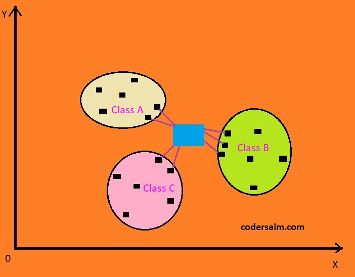
KNN stands for k-nearest neighbor. The k-nearest neighbor method is used to classify a new data point based on its k-nearest neighbor. In KNN classification if a new data point comes then it tries to find how many nearest neighbors are there around it. After getting the nearest neighbors its compares that how many neighbors are there from which class. New data points will be classified to that class, from which class most of the data points will come. Here k means that how many neighbors you want to compare. Suppose five data points are taken for k, then a new data point will find five nearest neighbors for classification. Always try to take odd values for k like 5,7,3 etc. To find which are the nearest data points it tries to find the distance between the new data point and other data points.
To find the distance it use,
two types method:
Formula of euclidean:
ED=√{(X₂-X₁)²+(Y₂-Y₁)²}
Manhattan
Formula: MD= [ | x B - x A | + | y B - y A |]
Any of these methods(Euclidean or Manhattan) can be used.

How KNN classifier works?

Suppose there are 2 class X and Y. X class have four data points A, B, C, D, and class Y have five data points F, G, H, I, J. A new data points come Z. Now find where the Z should go or in which class Z should belong. At first take k value as three. Now Z data point will try to find the three nearest data points from it. The distance will be measured by the euclidean distance finding technique. After getting the three nearest data points, now it will see that from which class most of the data points was came. For example, here 2 nearest data points are from class X and one data point is from class Y. Because most of the data points are from class X so Z data points will be classified as class X.

Support vector machine

What is Support vector machine?

The main idea of the support vector machine is that it finds the best splitting boundary between data. Here you have to deal with vector space, In this way, the separating line is a separating hyperplane. The maximum margin or space between classes is called the best-fitted line. The hyperplane is also called the decision boundary.

Some important concepts for support vector classifier:
Kernel: The kernel is a function that maps lower-dimensional data to higher-dimensional data. There are three types of kernel used, 1.Sigmoidal Kernel, 2.Gaussian Kernel,3.Polynomial Kernel etc.
Hyper Plane: In SVM hyperplane is the separation line between the data classes.
Boundary Line: In SVM there are two lines other than the Hyperplane which creates a margin. The support vectors can be on the boundary lines or outside them. This boundary line separates the classes.
Support vectors: Vector is used to define the boundary or vectors are those data points which help to define the boundary lines. These data points mean vectors lie close to the boundary.

How support vector machine works?

So you can have 2 types of data :

1.Linear data:
Linear data means the data which can be linearly separately or linear data means that type of data that can be separated by drawing a straight line.

How support vector machine works on linear data?

Think that there are two different types of data. Now draw a line between these two different types of data which will separate all the data and the drawn line known as a hyperplane.
Now there is a question that how to draw the line because the line can be drawn from anywhere.
To draw the best line find the maximum distance between classes and then have to find a midpoint point in that distance and then draw a line on that midpoint. Two sides of the hyperplane draw two boundaries.
How to draw boundaries?
For this find, a data point from each class which is so close to each other class and these points are called support vector. After finding those points draw a line which will do just a light touch those points. Draw lines to the parallel of the hyperplane. Now you have hyperplane and boundaries. So boundary means the nearest data of each class from the hyperplane. Now if you sum the distance of two boundaries from the hyperplane then you will get the margin. Always choose that point for creating a hyperplane where you get maximum width or distance between classes because the maximum width of margin gives better accuracy.

2. Nonlinear data:
Nonlinear data means the data which can't be linearly separate or nonlinear data means that type of data that can't be separated by drawing a straight line.

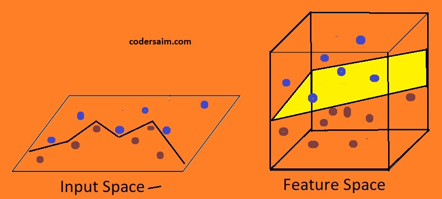
How support vector machine works on nonlinear data?

Because the data can't be separated by drawing a straight line so use kernel for classifying. So what the kernel does is that it take lower-dimensional data and convert it into higher dimensional data. The data you give to the kernel is nonseparable data means can't separate data by drawing a straight. It means now the data is in a lower dimension, but when you put the data in the kernel and when kernel converts our data into a higher dimension then the data becomes separable. It means that after converting the data from a lower dimension to a higher dimension then the data become linearly separable. Now you can linearly classify the data. Now the steps are the same for classification what you do in linearly data classification.

Random Forest Classifier

What is Random Forest Classifier?

Random forest is an ensemble bagging learning method. A decision tree is like a structured algorithm that divides the whole dataset into branches, which again split into branches and finally get a leaf node that can't be divided. Random forests creates multiple numbers of decision trees and these trees are called a forest. It means in decision tree we create one tree but in a random forest we create multiple trees and because there are too many trees so it is called a forest. To build a machine learning model the whole dataset is divided into train and test. Random forest takes data points from the training dataset and data points are taken randomly that's why it is called random forest.

Let's see an example:
Suppose you got a job offer letter from a company. After getting the letter you should ask someone who works in that company or know many things about that company like, is that company is good or bad, how much salary they will give, office rule, working rules, etc. Now if you make a decision depending on one person's opinion that may be not right. Because that person can be frustrated or very satisfied with the company. But if you ask too many people and then do vote everyone opinion and then taking a decision can be more accurate. So here you can compare taking opinions from one person with a decision tree and taking a decision from multiple people with random forest. The facilities of doing this are now the prediction will be more accurate. In a random forest, each tree will gives a predicted value and then you will do voting of all predicted values given by each tree and the result of the voting will be the output. You will get better Accuracy in the random forest to compare to decision tree

How Random Forest Classifier works?

sx Suppose there are 100 records in a dataset. Randomly take 25 records from that dataset and create a new small dataset or one bag, then again randomly take 25 data from the main dataset and create a 2nd bag or new dataset. Bags or new datasets will be created like this according to needs. Remember one thing, this selection is called replacement selection. It means that after creating one bag or one dataset from a random selection of data from the original dataset, the data you selected will go back in the main dataset again, and then again a new bag or new dataset will be created. It means bags can have duplicate records. It means the number one bag and number two bag can have the same records. Same records means all the data can't be the same, some data can be the same like number 1 record of the main dataset is present in all the bags or some bags and it also can be possible that number 1 record is present in only one bag. After creating the bags or small datasets the number of decision trees will be used equally to the number of bags or datasets. If 5 bags or mini datasets are created then 5 decision tree models will be used. After completing the training each model will give an output. Then combine all those model outputs and then do vote. which output is mostly predicted is the final output.

Naive bayes

What is Naive bayes?

Naive Bayes is a classification technique depending on the Bayes theorem or you can say a naive Bayes classifier guess the existence of a particular feature in a class is irrelevant to the presence of any feature. Its likelihood to that location where the existence of new dataset and take decision behalf of probability that where the data should go means which class it belongs to.

What is bayes theorem?

Bayes theorem is the probability of an event, depending on previous knowledge of conditions which can be related to the event.
Bayes theorem formula:P(A|B)={P(A) P(B|A)}/P(B)
Here,
P(A|B)= It is the probability of A according to B
P(A)= Probability of A
P(B)= Probability of B
P(B|A)=Probability of B according to A

How naive bayes works?

Let's think that you have two classes A, B, and a new data point C comes between these two data points. Find in which class the new data point should go. Class A has 10 data points and class B has 20 data points. The total number of data points is 30.
So,
P(A)=(class A data points)/(total data points)=10/30=0.33
It means the strength of class A is 0.33
P(C)=4/30=0.13
Here we find the strength of our new data point C. To do this create a circle and the number of data points comes in that circle, divide that with the total number of data points. In that circle data points can come from all classes or not from all classes but the new data point must have in that circle. Here 4 means 3 value comes from class A and 1 value comes from class B in that circle. The radius of the circle depends on you and the data points. Circle radius can be increased or decreased according to the need.
P(C|A)=3/10=0.3
P(A|C)=(0.3* 0.33)/0.13=0.75
Because 3 values from class a come in the circle that's why to divide 3 by the total number of data points of class A. Do the same work with class B
P(B)=20/30=0.66
P(C)=4/30=0.13
P(C|B)=1/20=0.5
P(B|C)=(0.5*0.13)/0.66=0.098
Here P(A|C)>P(B|C)
So the new data point will go to class A

How naive bayes work on bayes theorem?

Fruits	Yellow	Sweet	Long	Total
Orange	350	450	0	650
Banana	400	300	350	400
Others	50	100	50	150
Total	800	850	400	1200

In the dataset, you have different types of Fruits in the fruits column and some features like how many fruits are yellow sweet long. Find that which fruits is yellow, sweet, and long.
According to the formula:
P(A|B)={P(A) P(B|A)}/P(B)
At first we will do work for orange:
p(yellow|orange)={p(yellow)*p(orange|yellow)}/p(orange)
={(800/1200)(350/800)}/(650/1200)=0.5
P(Sweet|orange)={p(sweet)*p(orange|sweet)}/p(orange)
={(850/1200)(450/850)}/(650/1200)=0.69
P(long|orange)={p(long)*p(orange|long)}/p(orange)
={(400/1200)0}/(650/1200)=0
p(fruits|orange)=(0.5*0.69*0)=0

Then we will do work for Banana:
p(yellow|Banana)={p(yellow)*p(Banana|yellow)}/p(Banana)
={(800/1200)(400/800)}/(400/1200)=1
P(Sweet|Banana)={p(sweet)*p(Banana|sweet)}/p(Banana)
={(850/1200)(300/850)}/(400/1200)=0.75
P(long|Banana)={p(long)*p(Banana|long)}/p(Banana)
={(400/1200)(350/400)}/(4000/1200)=0.87
p(fruits|Banana)=(1*0.75*0.87)=0.65

Then we will do work for Others:
p(yellow|Others)={p(yellow)*p(Others|yellow)}/p(Others)
={(800/1200)(50/800)}/(650/1200)=0.04
P(Sweet|Others)={p(sweet)*p(Others|sweet)}/p(Others)
={(850/1200)(100/850)}/(650/1200)=0.66
P(long|Others)={p(long)*p(Others|long)}/p(Others)
={(400/1200)(50/400)}/(650/1200)=0.33
p(fruits|Others)=(0.04*0.66*0.33)=0.009

Here 0.87>0.009>0 means Banana>others>orange
So the result is Banana is that fruits which are yellow, long and sweet.

Naive bayes variants

Naive bayes can used in three ways:

BernoulliNBmport

Where BernoulliNBmport is used?
If the dataset features values are in binary natures then use BernoulliNBmport. Bernoulli distribution is used here.

How BernoulliNBmport works?
You have to learn two things:
1.P(1/success/yes)=p
2.p(0/failure/no)=1-p=q
If the values are in the binary form then you can have two types of values one is 1/yes/success/true/right etc and the other one is 0/no/failure/wrong/false etc. So here q is for the value of the negative types means 0/no/failure/wrong/false etc and p is for positive types value like 1/yes/success/true/right etc.
Now let's take a random variable X.If the random variable value is:
X=1 then it defines positive types value like yes/success/true/right etc. This defined as p.
and if
X=0 then it defines negative types value like no/failure/wrong/false etc. This is defined as 1-p=q.
Formula of BernoulliNBmport:
For X random variable the formula is,
p(X=x)=p^x*(1-p)^1-X
Here,
X=random variable
x= it can take two values 0 or 1
Now let's try solve the equation:
if x=0,
P(X=0)=p^0*(1-p)^1-0=1-p=q(here q is for negative types value like no/failure/wrong/false etc)
if x=1,
P(X=1)=p^1*(1-p)^1-1=p*1=p(here p is for positive types value like yes/success/true/right etc)
So this way BernoulliNBmport works with binary features.

GaussianNB

Where GaussianNB is used?
If the data have a continuous nature thenGaussianNB is used. Gaussian distribution or normal distribution is used.

What is gaussian distribution?
The shape of the gaussian distribution is the bell shape curve.
The formula of probability density function of gaussian distribution:
f(x)={1/√(2πσ)}*e^{-1/2σ^2}^(x-μ)^2
Here,
x=Random variable which ranging between -∞(Negative infinity) to +∞(Positive infinity)
μ=Mean
σ^2=Variance
σ=Standard Deviation

MultinomialNB

Where MultinomialNB is used?
Suppose there is a book page and you want to find a word frequency/discrete count/number of occurrences on that page. To do that you will use MultinomialNB. It means to find frequency/discrete count/number of occurrence MultinomialNB is used. Multinomial distribution is used in MultinomialNB. This model is widely used for document classification.